A Comprehensive Guide to Data Pre-Processing in Machine Learning

Introduction

Data pre-processing is essential to ensure that different algorithms can be effectively applied, stored, and retrieved for later use. The steps below will guide you through the process of data pre-processing.

Section A: Building Basics

“Build the basics strong, and you’ll go far without looking back.”

1. Features

Features are generally the columns in which different data is based. For example, in a company employee table, data like name, age, experience, salary, etc., are features that are shared among the employees to save that data in the database.

2. Independent Variables

These are variables that are independent of anything. For example, in the employee table mentioned earlier, name and age could be independent variables.

3. Dependent Variables

Dependent variables rely on independent ones. For example, the salary column could be dependent on factors such as experience and age.

4. Cleaning the Dataset

Cleaning datasets can be challenging, but it is crucial for improving the data quality. There are primarily two approaches:

4.1 Removing the Missing Row

If you have a large dataset, you can afford to remove rows with missing data using a Python library you are comfortable with.

4.2 Replacing with the Averages

When data is limited and important, you can replace missing values with the average of the column.

Note: Giving random or constant values to missing rows can increase the bias in the results.

5. Encoding Categorical Variables

For datasets with categorical variables, such as employee designations like IT, Business, and Marketing, encoding is necessary.

5.1 One Hot Encoding

Use one-hot encoding to convert categorical variables into vectors. For example, you can represent categories as [0, 0, 1], [0, 1, 0], and [1, 0, 0] in separate columns.

6. Training and Testing Set

The dataset should be split into a training set (used for training the model) and a testing set (used for validation). A common split is 80% for training and 20% for testing.

7. Feature Scaling

Feature scaling is essential for ensuring that features are on the same scale, which aids in comparison and improves model accuracy.

Types of Feature Scaling

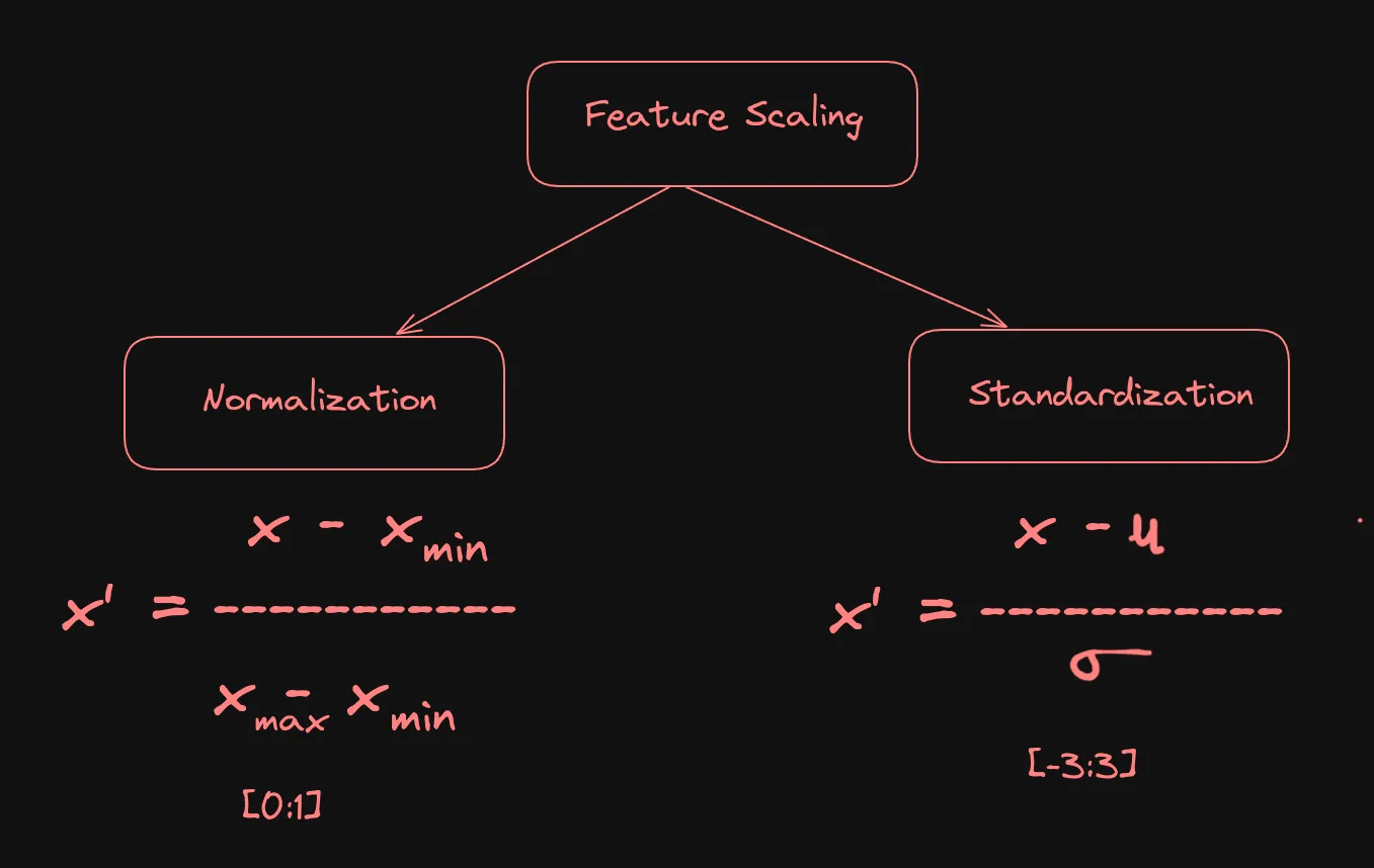
7.1 Normalization

Normalization is a technique used to scale numerical features between a specific range, usually between 0 and 1. This is helpful when different features have different scales, and it’s essential to compare or group them together. Normalization is commonly used when dealing with categorical data, such as image or audio data, where the values can vary significantly.

The formula for normalization is:

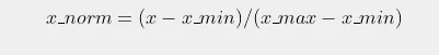
Where x is the original value, x_min is the minimum value in the dataset, x_max is the maximum value, and x_norm is the normalized value.

By using normalization, we can ensure that all features are on the same scale, which can improve the accuracy of machine learning models and help in better data comparison.ntly.

7.2 Standardization

Standardization does not have a fixed range of values. The resulting values follow a standard normal distribution with a mean of 0 and a standard deviation of 1. This means that the values can be any real number, but they will be centered around 0 and will have a relatively small spread. In practice, the values obtained after standardization can range from negative infinity to positive infinity, although they are most likely to fall within a few standard deviations of the mean. For example, if the standard deviation is 1, then 68% of the data will fall within one standard deviation of the mean (-1 to +1), 95% will fall within two standard deviations (-2 to +2), and 99.7% will fall within three standard deviations (-3 to +3).

Section B: Practical

1. Importing the Libraries

import numpy as np
import pandas as pd
import csv

Let’s assume our dataset is like this:

Designation	Months to Revenue	Revenue Generated (in thousands)	Revenue Profitable
Marketing	5	125	Yes
IT	2	160	Yes
Business	Nan	120	No
Marketing	4	150	Yes
IT	6	105	No
Business	3	Nan	Yes
Marketing	8	80	No
IT	5	125	Yes
Business	4	130	No
Marketing	3	210	Yes

2. Reading the CSV File

df = pd.read_csv("your_dataset_name.csv")
df

3. Splitting to X and Y

Y is the Output By looking at the dataset, we can see that Revenue Profitable column is the output that we want to predict. and X are the independent variables of the remaining columns.

X = df.iloc[:,:-1].values
Y = df.iloc[:, -1].values

4. Handling the Missing Data

Since we have a small dataset, we can’t afford to drop any of the rows with missing data, so we are filling that in with the averages.

from sklearn.impute import SimpleImputer

imputer = SimpleImputer(missing_values=np.nan, strategy='mean')
imputer.fit(X[:, 1:3])
X[:, 1:3] = imputer.transform(X[:, 1:3])

5. Encoding Categorical and Independent Variables

from sklearn.compose import ColumnTransformer
from sklearn.preprocessing import OneHotEncoder

ct = ColumnTransformer(transformers=[('encoder', OneHotEncoder(), [0])], remainder='passthrough')
X = np.array(ct.fit_transform(X))

6. Encoding the Dependent Variable

Since it has only two labels, Yes or No. So, we are applying this LabelEncoder to the dependent variable.

from sklearn.preprocessing import LabelEncoder

le = LabelEncoder()
Y = le.fit_transform(Y)

7. Splitting the Dataset into Training and Testing Set

from sklearn.model_selection import train_test_split

X_train, X_test, Y_train, Y_test = train_test_split(X, Y, test_size=0.2)

8. Applying Feature Scaling

We don’t need to apply the feature scaling to the categorical variables that we encoded earlier; it can make those worse. We generally do feature scaling to keep the same scale overall. We need to apply the same transform to the train as well as the test.

from sklearn.preprocessing import StandardScaler

sc = StandardScaler()
X_train[:,3:] = sc.fit_transform(X_train[:,3:])
X_test[:,3:] = sc.transform(X_test[:,3:])

Conclusion

Data pre-processing is a crucial step in the data science pipeline. It ensures that data is clean, well-formatted, and ready for analysis, which improves the performance of machine learning models. By following the steps outlined in this guide, you can now transform raw data into a structured format that is suitable for various analytical tasks. If you really loved this, be sure to follow me, and thanks for reading. Have a great day.